An Introduction to Gnuplot
Introduction
Gnuplot is an incredibly powerful and useful utility for presenting data in graphical format. In this post I’ll cover a very simple usecase that involves graphing the size of a database over a period of time.
Installing
On Linux use your normal package manager, e.g.
# Debian based...
apt-get install gnuplot

# Redhat based...
yum install gnuplot
The easiest way to install gnuplot on OS X is using brew. Gnuplot requires X11 to display graphs so to install it use,
brew install gnuplot --with-x11
If X11 support isn’t available gnuplot will fail to display graphs with the error,
WARNING: Plotting with an 'unknown' terminal.
No output will be generated. Please select a terminal with 'set terminal'.
If this happens uninstall and then reinstall with X11 support.
Basic Usage
In the example below I’ll use a data file called db_size.dat. Each line in this file records the size of a database at an hourly interval.
The most basic gnuplot command to graph this data would be,
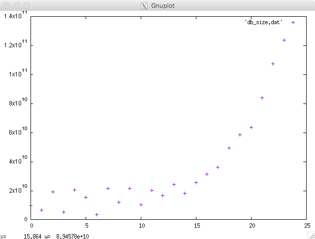
gnuplot -p -e "plot 'db_size.dat'"
The -p parameter (short for persist) leaves the window containing the graph open after gnuplot finishes.
The -e parameter is the command to pass to gnuplot. The command plot 'db_size.dat' means plot a graph using the data in db_size.dat.
Running this command will open a a window with this graph.
Depending on your requirements this simple graph may be absolutely fine. However if you’d like to polish it up there are a few changes we can make.
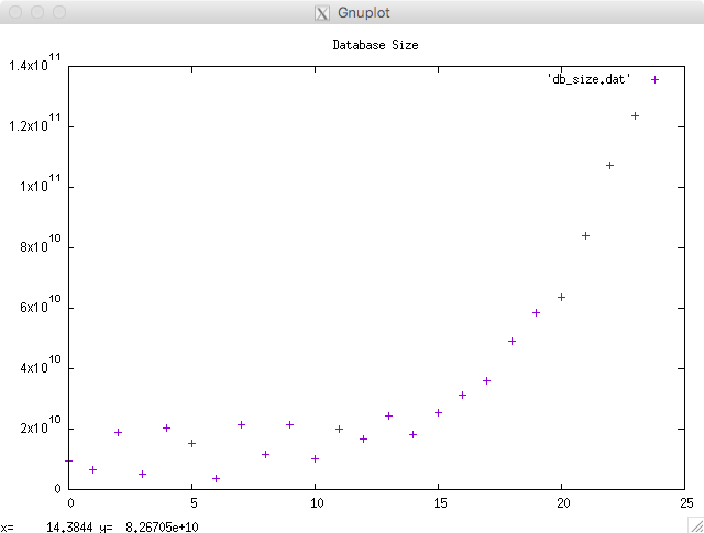
First of all lets give the graph a title.
gnuplot -p -e "set title 'Database Size'; plot 'db_size.dat'"
At this stage the command line is getting a little long. This is where gnuplot command files come into play. Each file is basically a list of commands.
This command file is called ‘db_size.gnuplot’,
set title 'Database Size'
plot 'db_size.dat'
The command file name is passed to gnuplot as a parameter,
gnuplot -p db_size.gnuplot
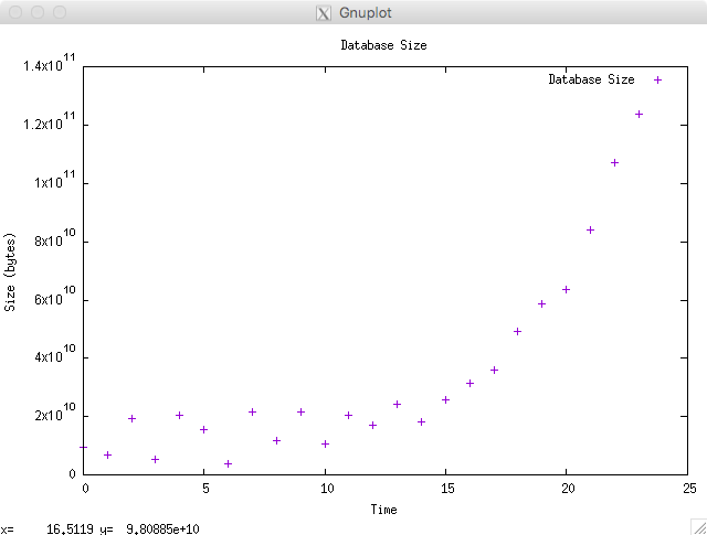
Lets add axis labels and give the key a name.
set title 'Database Size'
set xlabel "Time"
set ylabel "Size (bytes)"
plot 'db_size.dat' title 'Database Size'
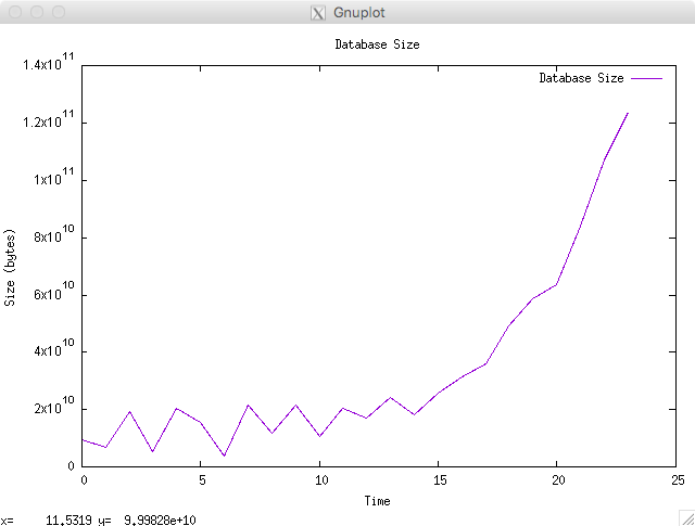
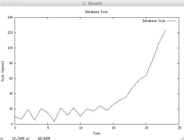
The dots can be difficult to follow when the they’re spaced out so lets use a line instead.
set title 'Database Size'
set xlabel "Time"
set ylabel "Size (bytes)"
plot 'db_size.dat' title 'Database Size' with line
The last change I’d like to make is to make the Y-axis scale more readable by converting bytes to gigabytes.
set title 'Database Size'
set xlabel "Time"
set ylabel "Size (GB)"
plot 'db_size.dat' using ($1/1000000000) title 'Database Size' with line
Finally lets save the graph to a PNG rather than displaying it on screen.
set term png
set output "db_size.png"
set title 'Database Size'
set xlabel "Time"
set ylabel "Size (GB)"
plot 'db_size.dat' using ($1/1000000000) title 'Database Size' with line
This saves the graph to a file called db_size.png in the current directory.
Going a Little Further
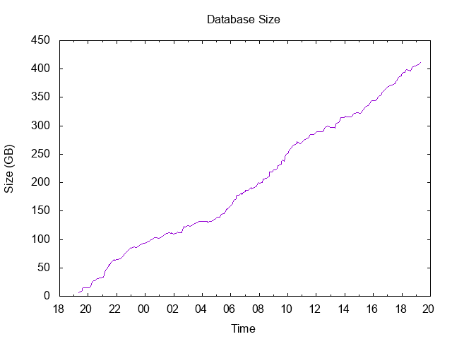
In the previous example there was one data value recorded at fixed intervals, i.e. hourly. But what if the same data is collected at irregular intervals? To reliably graph this data we need to record the time each data point is recorded, db_size_with_time.dat. In this file the first column is seconds since the epoch. Gnuplot can parse this using the ‘set xdata’ command. Here’s the full command file,
set title 'Database Size'
set xlabel "Time"
set ylabel "Size (GB)"
set key off
set xdata time
set timefmt "%s"
set xtics format "%H"
plot 'db_size_with_time.dat' using 1:($2/1000000000) with line
set key offturns off the key. Its not very useful in this graph.set xdata timeparses the X axis data as a time.set timefmt "%s"means read time values as seconds since the epoch.set xtics form "%H"means write the hour to the X axis
This post barely scratches the surface of what can be achieved using gnuplot. It’s really an amazing piece of software.
For more information: